We love it when our API comes in useful for academic purposes. This is a guest post by Richard Thomas.
For my MSc dissertation, I investigated determinants of the proportion of people who choose to cycle for their daily commute. Specifically, I wanted to see whether an analysis of realistic cycling routes of a representatively large sample of a city’s population could give improved predictors over existing models.
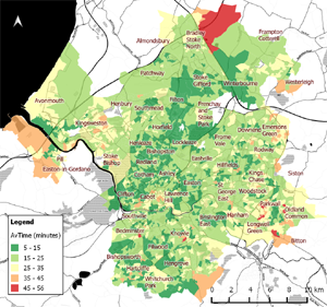
From 2011 Census data, I extracted commuting origin/destination data for everyone in the Bristol built-up area in its most detailed form of aggregation (typically accurate to within 500m). I wanted to generate plausible cycling routes for these commutes, then for each of these routes to evaluate metrics (distance, hills, cycle paths, traffic). As census data is available giving the proportion of commuters living in each small area who cycle, multi-variate correlation could then be used to estimate the influence of these routing metrics, together with other known influential population measures taken from the census.
So how best to perform this cycle routing and evaluate suitable metrics? On both these counts the CycleStreets Journey Planner API proved invaluable (and made my MSc dissertation a feasible proposition!) I had considered using an existing open source routing engine (such as pgRouting or Graphhopper) operating on an extract of the OpenStreetMap database as this would allow me to directly query tags on each node of a route. However the complexity in interpreting OpenStreetMap cycle-related tags is quite daunting (as documented here on CycleStreets.net).
Because the API returned not just the route, but details of routed distance, duration, “quietness”, estimated calories required and spot heights, useful metrics could be derived quickly from the JSON data using just Python scripts. It would have been good to more directly quantify dedicated cycle infrastructure along routes: although the “quietness” measure included this, it also included road traffic expectations. Given more time, this could have been done by using the actual route coordinates to interrogate the OpenStreetMap or CycleStreets databases, though this was complicated by API-returned points being only in latitude/longitude format rather than database node/segment numbers. In order to limit the amount of data to be processed (and the load on the CycleStreets API server, routing was limited to the 4 most popular routes from each area, although this still required nearly 16,000 routes to be generated and analyzed!
The most notable results of these new routing-based metrics (i.e. beyond the key predictor of crow-fly distance) were as follows:
- Directness (Crow-fly / Routed Distance): strong indication that cycling was less popular if a reasonable (“balanced”) cycling route was particularly circuitous.
- Max Height Increase (Maximum of sum of all hill climbs for outward or return direction): strong indication (as might be expected) that hills were a strong detractor. This metric was only developed after the MSc was completed; interestingly, in the MSc analysis, the related metric of Effort Ratio (calories / distance) was not a statistically significant indicator.
- Traffic Exposure (Inverse of “Quietness”): Although this metric visually gives a good indication of cycling routes along busy roads and/or away from dedicated cycle infrastructure it was not a statistically significant predictor of cycling. Although not conclusive, this supports other research showing that cyclists are more sensitive to time taken than to pleasantness or safety when it concerns their daily commute (priorities may be different for a leisure ride).
More details of the analysis are available in the full dissertation (or short synopsis). Detailed 2011 census origin/destination data (table WF02 for OA/WZ) was only made available after the end of my MSc (and then only to academics for specific projects). Thus for the MSc, synthetic data was generated based on (publicly available) census data. However, a later reworking of the full analysis using the new WF02 census data gave very similar results showing that lack of public access to detailed statistics need not be a serious impediment to analysis.
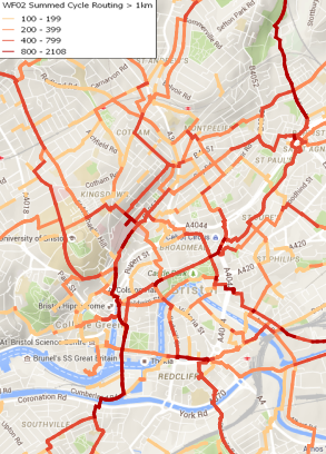
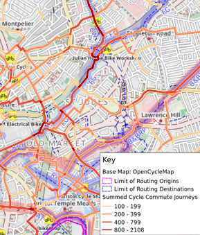
Beyond the key MSc analysis, an interesting spin-off of all the cycle routing was the development of maps (see right and below) that sums the 4 most popular commute routes from the centroid of each census Output Area, giving a good indication of the number of cyclists along individual streets if all these people were to commute by bicycle.
Thanks again to CycleStreets for making the API available to enable this research project. Data processing was done in Python and SPSS with additional processing and map rendering in the open source QGIS package.
Richard Thomas
Editor’s note: We now have a batch routing system available which we’re keen to encourage for academic use like this. It can handle millions of combinations happily – not just the 16,000 combinations noted above!


